
(2/2) 7 Flink Internals That Explain How It Processes 80 Million Events Per Second Without Dropping A Single Record
Most Flink tutorials show you the API. This one shows you what's running underneath it.

Part 1 covered Flink’s streaming-first philosophy, system architecture, dataflow execution, and stream analytics including time, watermarks, and windowing. If you missed it, the link is at the bottom.
Part 1 built the foundation. You understand why Flink was designed the way it is, how data moves through the execution graph, and how it thinks about time. The natural next question is what happens when that execution breaks down.
A node fails. A network partition occurs. A process crashes at exactly the wrong moment. In a stateful system processing millions of events per second, any of these can corrupt results in ways that are nearly impossible to debug after the fact.
The next three sections go into the engine room. Fault tolerance, batch optimization, and native iteration. This is where Flink’s claim of being a unified engine either holds up or falls apart.
5. Fault Tolerance and State Management
Flink’s answer to failure is one of the most carefully designed pieces of engineering in the entire system.
5.1 Asynchronous Barrier Snapshotting
The core challenge with fault tolerance in a distributed streaming system is taking a consistent snapshot of every operator’s state simultaneously without pausing the pipeline.
Pausing works but is unacceptable in production. For a fraud detection system or a real-time bidding pipeline, a pause is the product failing.
Flink’s solution is called Asynchronous Barrier Snapshotting. The data never stops flowing, and that single property is what makes the mechanism work.
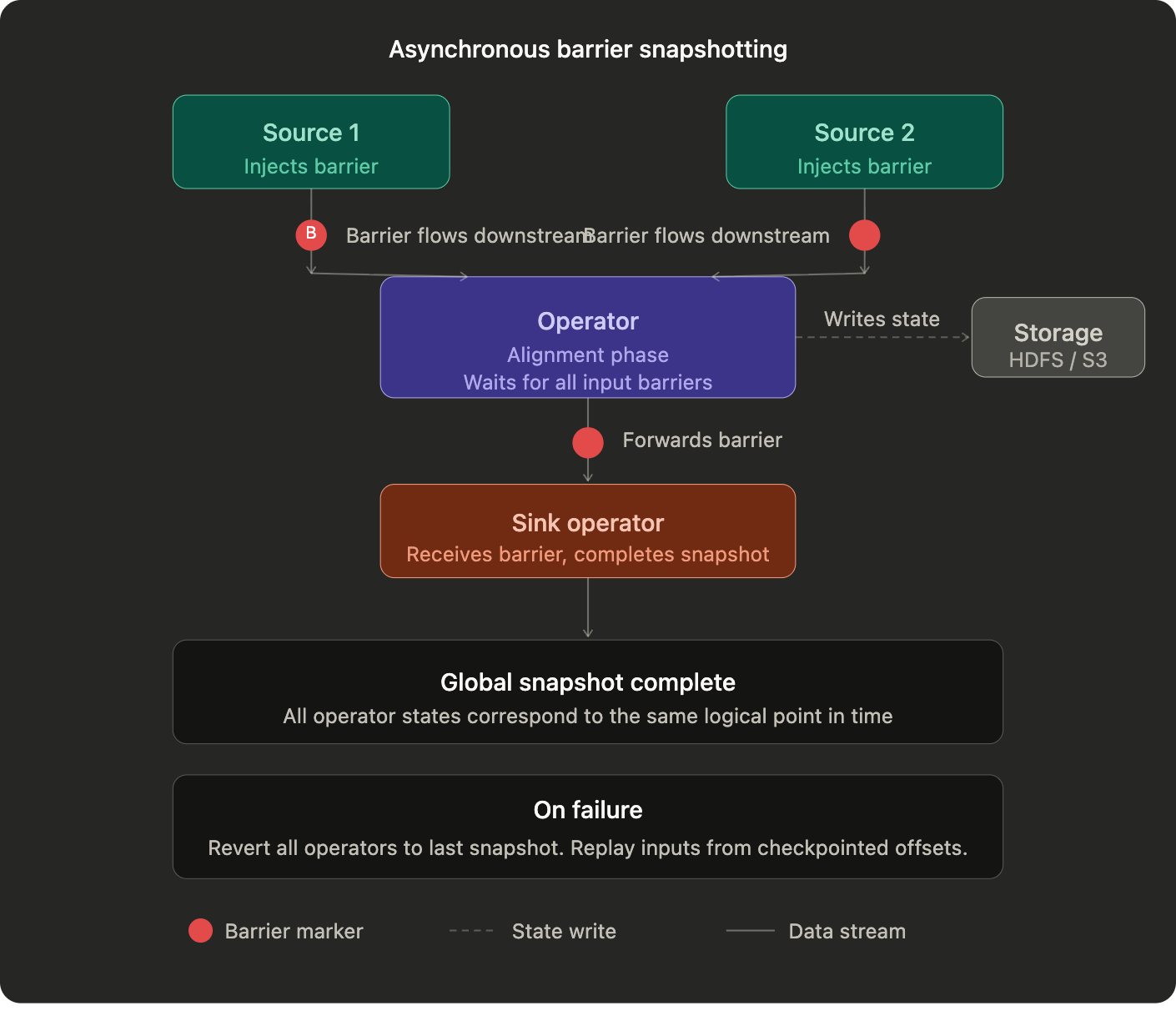
The JobManager periodically injects special control records called barriers into every input stream. If the word “control records” sounds familiar, it should. Barriers use the same control event mechanism as watermarks, which you saw in Part 1. Just as watermarks signal progress in event-time, barriers signal progress in snapshot coordination. A barrier is an invisible marker that travels downstream alongside your actual data records, carrying one piece of information: a snapshot ID.
When an operator receives a barrier from an upstream partition, it waits until barriers from all of its input partitions have arrived. This is the alignment phase. While waiting, the operator keeps processing records from partitions whose barriers have already arrived and buffers records from partitions that have not yet sent their barrier. Once all barriers are aligned, the operator writes its current state to durable storage, processes the buffered records, and forwards the barrier downstream. Eventually every operator in the DAG completes this process and a global consistent snapshot exists.
The result: snapshots contain only operator states, kept to the theoretical minimum size, taken without interrupting execution. And because every operator’s state corresponds to the same logical point in time, that snapshot is the foundation for exactly-once guarantees.
5.2 Exactly-Once Guarantees
ABS gives Flink something most streaming systems cannot credibly offer: exactly-once processing guarantees.
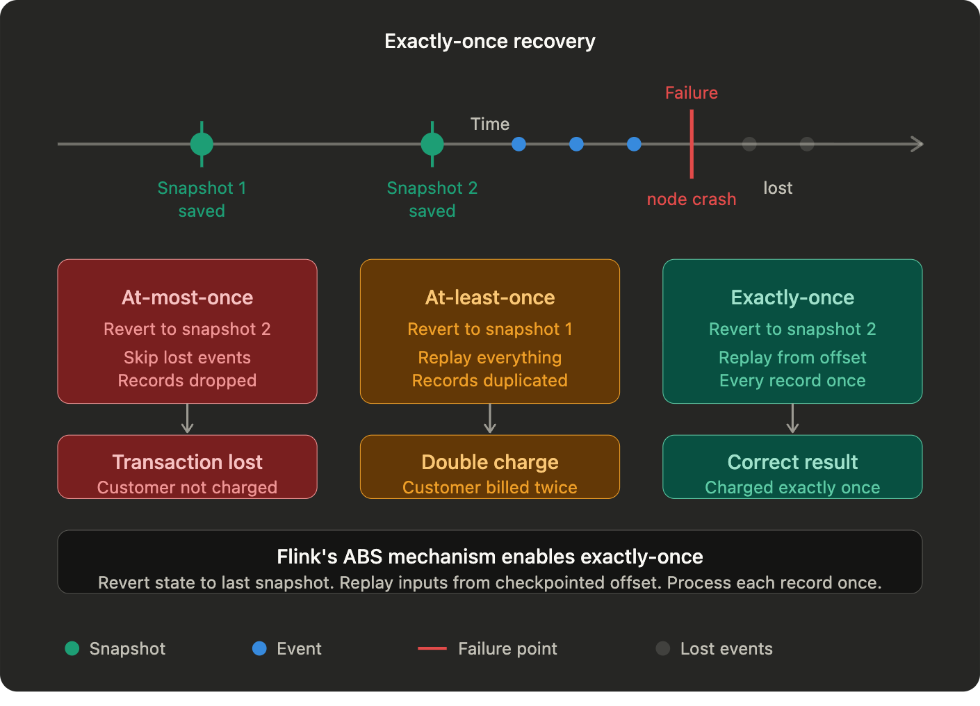
Not at-least-once, where a record might be processed multiple times after a failure. Not at-most-once, where records might be dropped. Exactly once. Every record affects the output exactly one time regardless of how many failures occur.
The practical consequence is direct. In a billing system, at-least-once processing means a customer gets charged twice after a recovery event. At-most-once means a transaction disappears entirely. Exactly-once is not a nice-to-have in financial, compliance, or any system where record-level correctness is a product requirement. It is the baseline.
When a failure occurs, Flink identifies the most recent successful snapshot. It reverts every operator’s state to what it was at that point and restarts input streams from the position recorded in the snapshot. For a Kafka source, this means replaying from the exact offset that was checkpointed. Kafka makes this possible because it is designed to retain the raw event log on disk, independently of whether any consumer has read it. The maximum recomputation needed is bounded by the interval between two consecutive barriers. Everything before the last snapshot is already durably stored.
One important nuance: exactly-once guarantees require that your sources are persistent and replayable. For sources that cannot replay, Flink can maintain a write-ahead log inside the source operator’s state, storing unprocessed events within Flink itself until the next checkpoint clears them. This works but comes at a cost: instead of storing a handful of offsets, Flink now stores raw event data, which becomes expensive at scale. That is why replayable sources are an architectural recommendation, not just a preference.
5.3 Managed State
State in most streaming systems is an afterthought. You manage it yourself in an external database or cache. When something fails, reconciling that external state with your pipeline’s position is your problem.
Flink takes the opposite approach. State is a first-class citizen in the API.
When you write a Flink operator you declare your state explicitly and register it with the framework. Flink then owns it completely: it partitions state by key, stores it durably, includes it in every checkpoint, and restores it automatically on recovery.
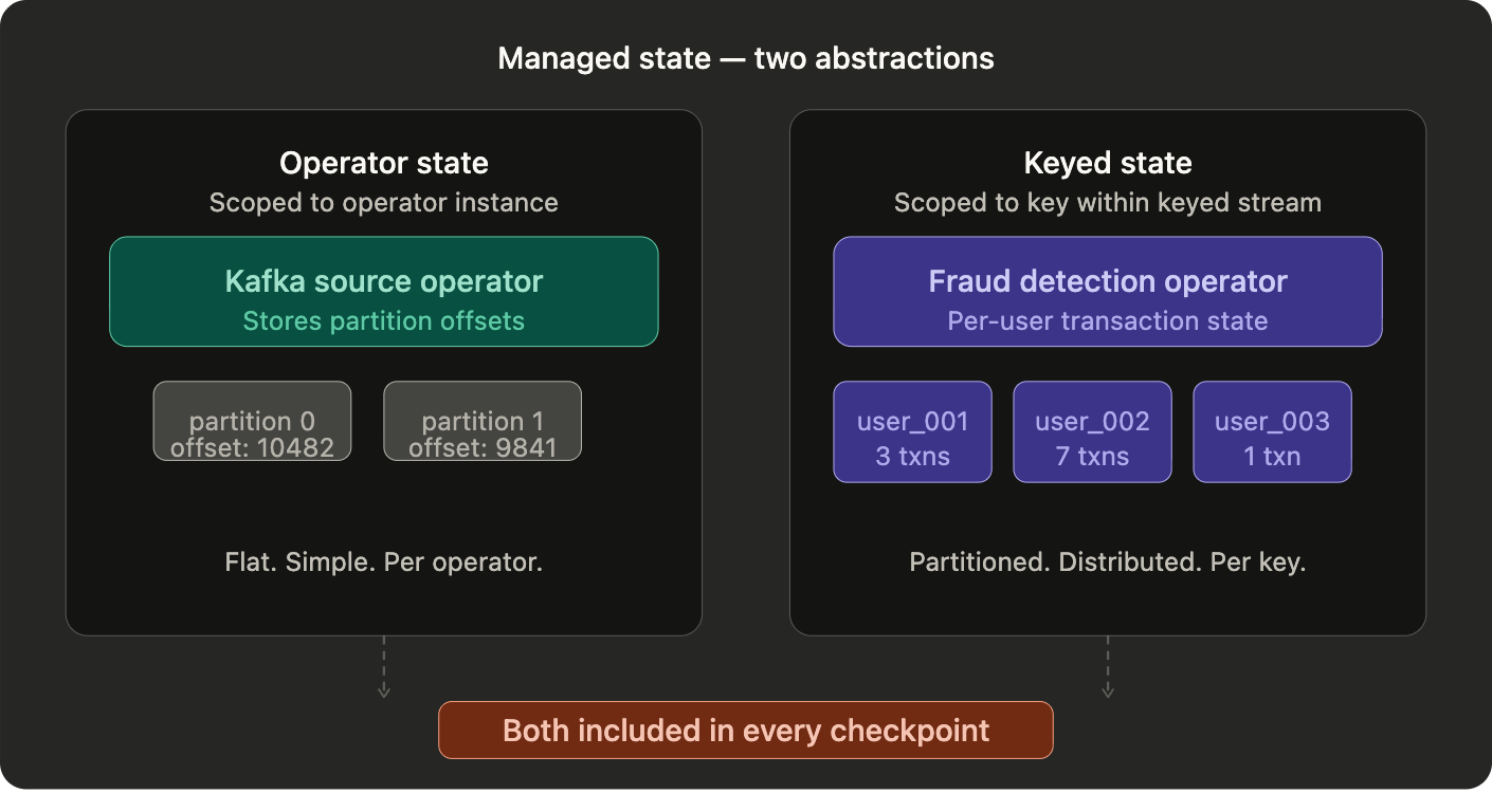
Two abstractions handle this. Operator state is scoped to an operator instance. A Kafka source uses this to store its partition offsets. Flat, simple, and tied to the operator itself. Keyed state is scoped to a specific key within a keyed stream. For every unique key flowing through your pipeline, Flink maintains an independent state entry. A session management system tracking active user sessions stores one state entry per session ID. Flink handles the partitioning, distribution, and recovery of all of it transparently.
The underlying storage is configurable through the StateBackend abstraction. For state under a few gigabytes, JVM heap storage gives you the lowest access latency. For state that exceeds memory bounds or needs to survive TaskManager restarts independently, RocksDB is the right choice. RocksDB is an embedded key-value store that spills to disk automatically when memory fills up. The operator code does not change based on which backend you choose. Only the configuration does.
Making state explicit means Flink’s checkpointing mechanism can guarantee that any registered state is durable with exactly-once update semantics. The pipeline does not just recover. It recovers to a state that is provably correct.
6. Batch Analytics and Optimization
Streaming is where Flink earns its reputation. But a system that handles batch poorly is not a unified engine. It is a streaming system with batch bolted on as an afterthought.
Flink treats batch as a genuine first-class workload. Two design decisions make that claim credible: a cost-based query optimizer that chooses execution strategies the way a database would, and a memory management model that sidesteps one of the most painful failure modes in the JVM ecosystem entirely.
6.1 Query Optimization
When you submit a batch job through the DataSet API, something happens before a single record is processed. The client runs your program through a query optimization pass.
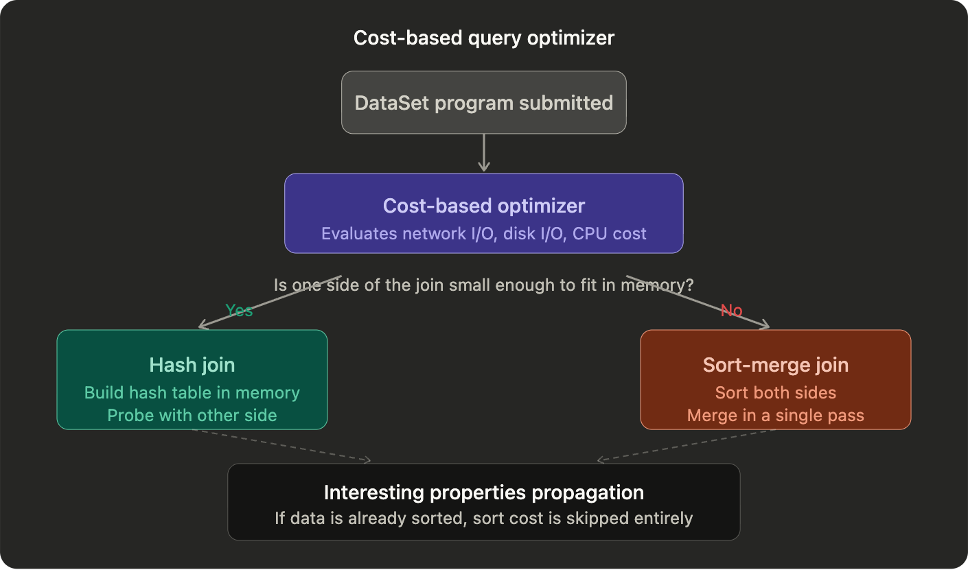
This is the same class of optimization that relational databases have spent decades perfecting. Flink’s optimizer evaluates multiple physical execution plans for your job and picks the one with the lowest estimated cost, accounting for network I/O, disk I/O, and CPU together.
The most consequential decisions it makes are around joins. A concrete example before the mechanics: if your data is already sorted by user ID from a previous groupBy operation and your next operation is a join on user ID, the optimizer recognises that and skips the sort entirely. On a large dataset that is the difference between a job that runs in 10 minutes and one that runs in 40.
The two physical strategies it chooses between are a hash join and a sort-merge join. A hash join builds an in-memory hash table from one side of the join and probes it with records from the other side. Fast when one side fits in memory, expensive when it does not. A sort-merge join sorts both sides independently and merges them in a single pass. More memory-resilient, but the sort cost is significant unless the data is already ordered.
This is where interesting properties propagation becomes important. Flink’s optimizer tracks whether data is sorted, partitioned, or grouped in a way that benefits downstream operators. If a sort produced in one stage can be exploited by a join in the next, the optimizer avoids re-sorting. It propagates these properties through the entire execution plan and uses them to eliminate redundant work at every stage.
The one constraint the optimizer works around: your operators are arbitrary user-defined functions. A SQL database knows exactly what a WHERE clause does to data properties. Flink does not know what your custom map function does. To handle this, Flink allows programmers to provide hints the optimizer can use when it cannot infer properties automatically.
The result is that batch jobs submitted through the DataSet API are not just executed. They are planned, the way a query planner would, before execution begins.
6.2 Memory Management
Every engineer who has run a large JVM application has encountered this at some point.
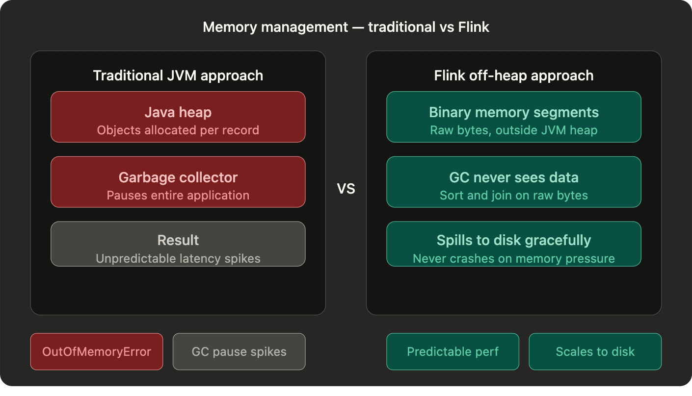
Your job is processing a large dataset. Memory fills up. The garbage collector kicks in. For a fraction of a second, sometimes several seconds, your application pauses while the GC reclaims heap space. At scale these pauses become unpredictable, latency spikes, and in the worst case your job fails with an OutOfMemoryError on a dataset you were confident your cluster could handle.
Flink sidesteps this problem entirely with a different approach to memory management.
Rather than allocating Java objects on the JVM heap to represent data records, Flink serializes data directly into fixed-size binary memory segments. These segments live off-heap, outside the garbage collector’s jurisdiction. The GC never sees them.
Operations like sorting and joining work directly on this binary representation wherever possible. A sort does not deserialize records into Java objects, sort them, and serialize them back. It operates on the raw binary data, comparing and reordering byte sequences directly. Deserialization only happens when the operator actually needs to read a field value, not when shuffling data around.
Two consequences follow. GC pauses become short and infrequent because the GC is not managing the bulk of your data. And when a batch operation exceeds its memory bounds, Flink spills the binary data to disk rather than failing. The job slows down but continues. A job that takes twice as long is almost always preferable to a job that crashes and forces a full restart.
For engineers running large batch jobs: you can process datasets significantly larger than your available heap memory, on the order of hundreds of gigabytes on a modest cluster, without tuning GC parameters, adjusting heap sizes, or debugging OutOfMemoryErrors. The memory model handles it for you.
7. Native Iterative Processing
Most data processing is linear. Data enters, transforms, exits. But an entire class of algorithms does not work this way.
Machine learning model training. Graph analytics. Gradient descent. PageRank. These are fundamentally iterative: they run the same computation repeatedly, feeding the output of one round back as the input to the next, until the result converges.
How a system handles iteration reveals a lot about how seriously it was designed for real-world workloads.
7.1 Feedback Loops
The naive approach to iteration in a distributed system is to submit a new job for each round. Run the computation, write the output to disk, submit a new job that reads that output, repeat until done.
This works. It is also expensive. Each job submission carries overhead. Each round requires writing intermediate results to disk and reading them back. For an algorithm that needs hundreds of iterations, which gradient descent often does, that overhead compounds into something that makes the approach impractical at scale.
Flink’s approach is different. Iterations are implemented as cyclic dataflows: special operators that contain their own execution graph and establish a feedback channel back to the start of the iteration step.
Two special task types make this work. The iteration head task establishes the feedback channel and controls entry into the iteration. The iteration tail task sits at the end of the iteration step and feeds results back to the head for the next round. The coordination between them uses the same control event mechanism as barriers and watermarks, so the iteration system integrates cleanly with the rest of the execution model rather than being bolted on separately.
Intermediate results never leave the TaskManagers between iterations. No disk write between rounds. No job resubmission overhead. The data stays in memory and the computation loops natively within the running job.
Flink supports two models for structured iterations. Bulk Synchronous Parallel requires all tasks in an iteration step to complete before the next step begins. It gives you exact deterministic results and is the right choice for algorithms like shortest paths where a stale update would produce a wrong answer. Stale Synchronous Parallel allows faster tasks to proceed ahead of slower ones within a bounded lag. It trades exactness for throughput and is the right choice for algorithms like gradient descent where a slightly stale weight update is acceptable and convergence speed matters more than precision.
7.2 Delta Iterations
Bulk iterations have a subtle inefficiency that becomes significant at scale.
In many iterative algorithms, only a small fraction of the data changes between rounds. A graph algorithm computing shortest paths updates only the nodes whose shortest path improved in the last round. A machine learning model training on sparse features updates only the weights corresponding to non-zero features in the current batch.
Bulk iterations do not exploit this. Every round processes the full dataset regardless of how much actually changed. For a graph with 100 million nodes where only 50,000 update in a given round, you are doing 2,000 times more work than necessary.
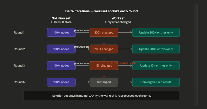
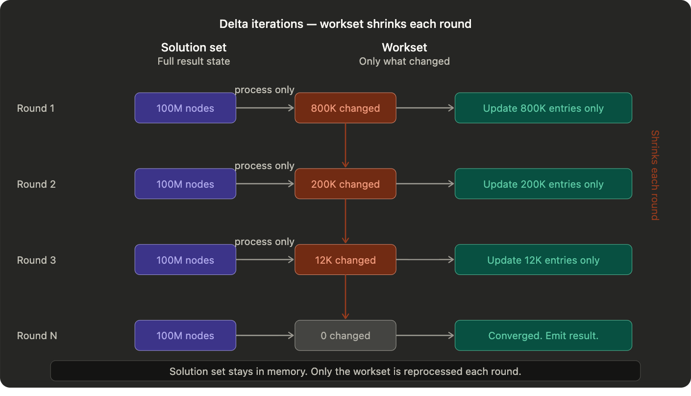
Delta iterations solve this by splitting the dataset into two parts. The solution set holds the current state of the full result, updated in place across iterations. The workset holds only the subset of data that changed in the last round and needs to be processed in the next one.
At the start of each iteration, only the workset is processed. The solution set is updated only for the elements touched by the current workset. The next workset contains only the elements that changed in the current round. The iteration terminates when the workset becomes empty, meaning nothing changed and the algorithm has converged.
As the algorithm converges the workset shrinks. Each successive round is cheaper than the last. The savings compound.
Flink’s graph library Gelly is built directly on top of delta iterations. Every algorithm in it, connected components, single-source shortest paths, label propagation, exploits this mechanism automatically. The savings are not something you implement. They are baked into the execution model.
Seven sections. Two parts. One execution model that handles real-time streams, batch workloads, stateful computations, and iterative algorithms without ever switching engines.
Most systems solve one of these problems well. Flink was designed from first principles to solve all of them. Understanding why it is built the way it is means you can now make that architectural decision with your eyes open rather than based on a benchmark someone else ran on a dataset that looks nothing like yours.
This breakdown is based on the original Apache Flink paper: “Apache Flink: Stream and Batch Processing in a Single Engine” by Paris Carbone, Asterios Katsifodimos, Stephan Ewen, Volker Markl, Seif Haridi and Kostas Tzoumas. Published in the IEEE Computer Society Technical Committee on Data Engineering Bulletin, 2015. Read the full paper here.
Part 1 of this series: Link.
Have a great day :)